Scarlatti: In-memory Hypergraph Machine Learning
| Id | Status | Submission Date | Grant Date | Authorship |
|---|---|---|---|---|
| 18/492,418 | Granted | 23 Oct 2023 | 12 Aug 2025 | 100% |
Imagine having an enormous collection of interconnected facts, like a knowledge graph. Now, imagine you want to find very specific patterns within this data. Not just simple searches, but complex relationships. The challenge is, how do you tell a computer exactly what to look for without writing incredibly complicated instructions every single time?
This is where the method comes in. It helps computers automatically create powerful search programs (called Query Programmes, or QPs) to dig out exactly the information you need from a special kind of database called an in-memory hypergraph knowledge base (KB).
Learning from Examples
You show the system:
• Positive samples (+S): Examples of the information you do want to find.
• Negative samples (-S): Examples of the information you do not want to find.
The method’s job is to build a QP that, when run, will find all your “wanted” examples and ignore all the “unwanted” ones. This might sound simple, but finding the perfect solution can be incredibly hard, like looking for a needle in a haystack where the haystack is constantly growing and changing. It’s a problem known to be very complex, but this method uses a smart, shortcut approach (a “heuristic”) to drastically speed up the search and find solutions efficiently.
What Exactly is a Hypergraph?
To understand how it works, let’s briefly explain what a hypergraph is. Think of it as a more flexible version of a typical graph (like the ones with circles and lines connecting them). In a standard graph, a line usually connects just two items.
However, in a hypergraph, a single connection (called an “edge”) can link any number of items (called “vertices”). This makes them incredibly versatile for representing complex data:
• They can describe RDF stores, where connections link a subject, a relationship, and an object.
• They can also represent rows in a standard database table, where each row’s elements are connected by an edge.
The method works with “labelled, indexed hypergraphs”. This means each connection has a type (like isA for “is a type of,” or partOf for “is a part of”), and each item within a connection has a specific order or position. For example, a query might look like:
partOf(X0,X1),isA(X0,capital),isA(X1,country)
Why this method is efficient?
Several core ideas make this system effective:
• Built for Hypergraphs: Unlike general graph methods, this approach is specifically tailored for hypergraph knowledge bases, giving it a much broader reach and efficiency for complex data relationships.
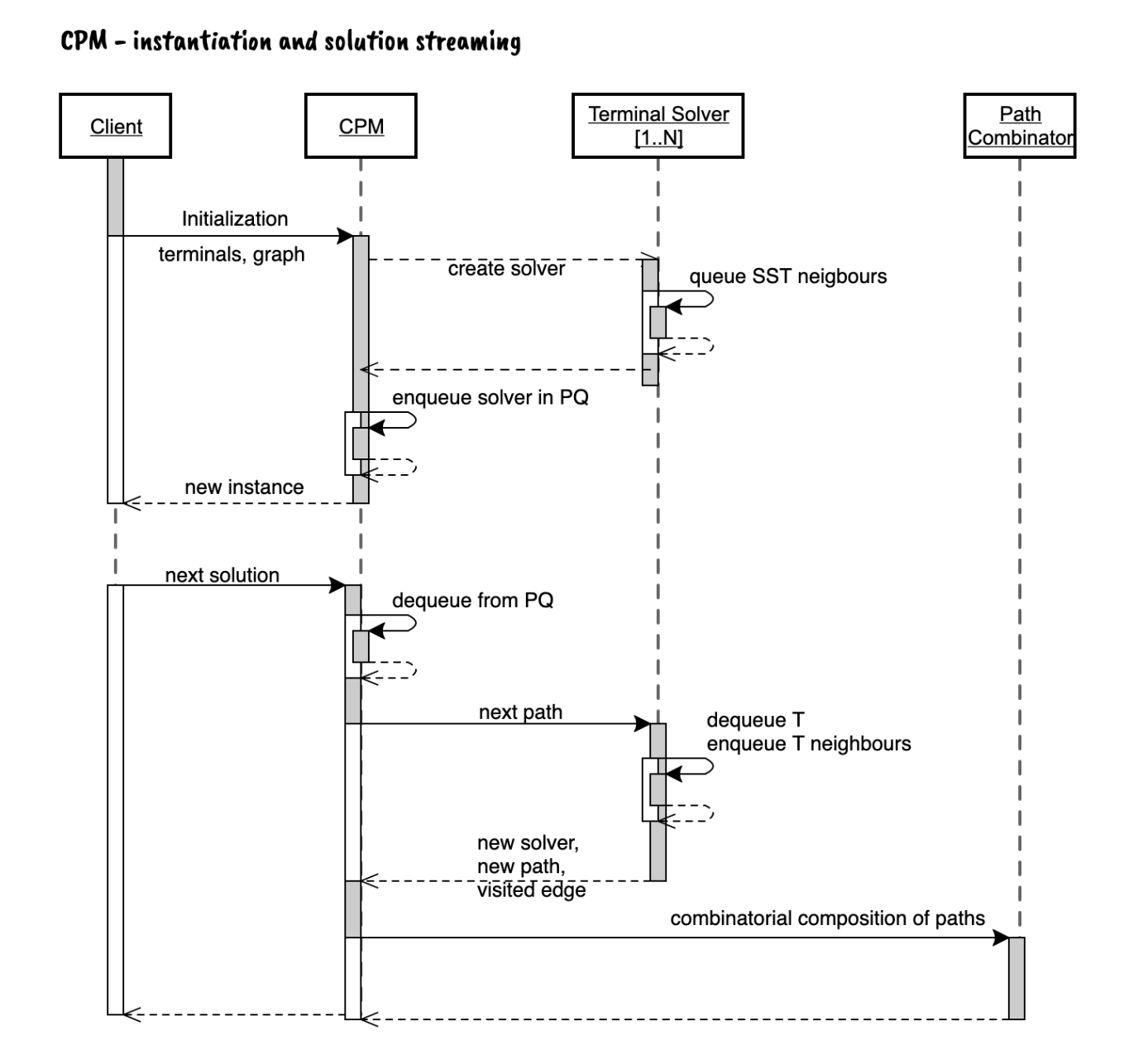
• “lazy stream” Solutions: Solutions are delivered as a “lazy stream”. This means the system only calculates parts of the solution when they are actually needed. If it finds a perfect solution right away, it doesn’t waste time looking for any others. The same lazy evaluation principle is applied in the combinatorial problem solver, where solutions are streamed on demand.
• Shortest Solutions First: The system prioritises finding the QP that involves the fewest connections or operations. Simpler queries are often better.
• Maximising Generalisation: A key goal of machine learning is to synthesise solutions that not only meet your specific examples but also work broadly for new, unseen data. The method achieves this by keeping queries “open” – using general “variables” in the query whenever possible, rather than fixed values, unless a fixed value is absolutely necessary to match your requirements.
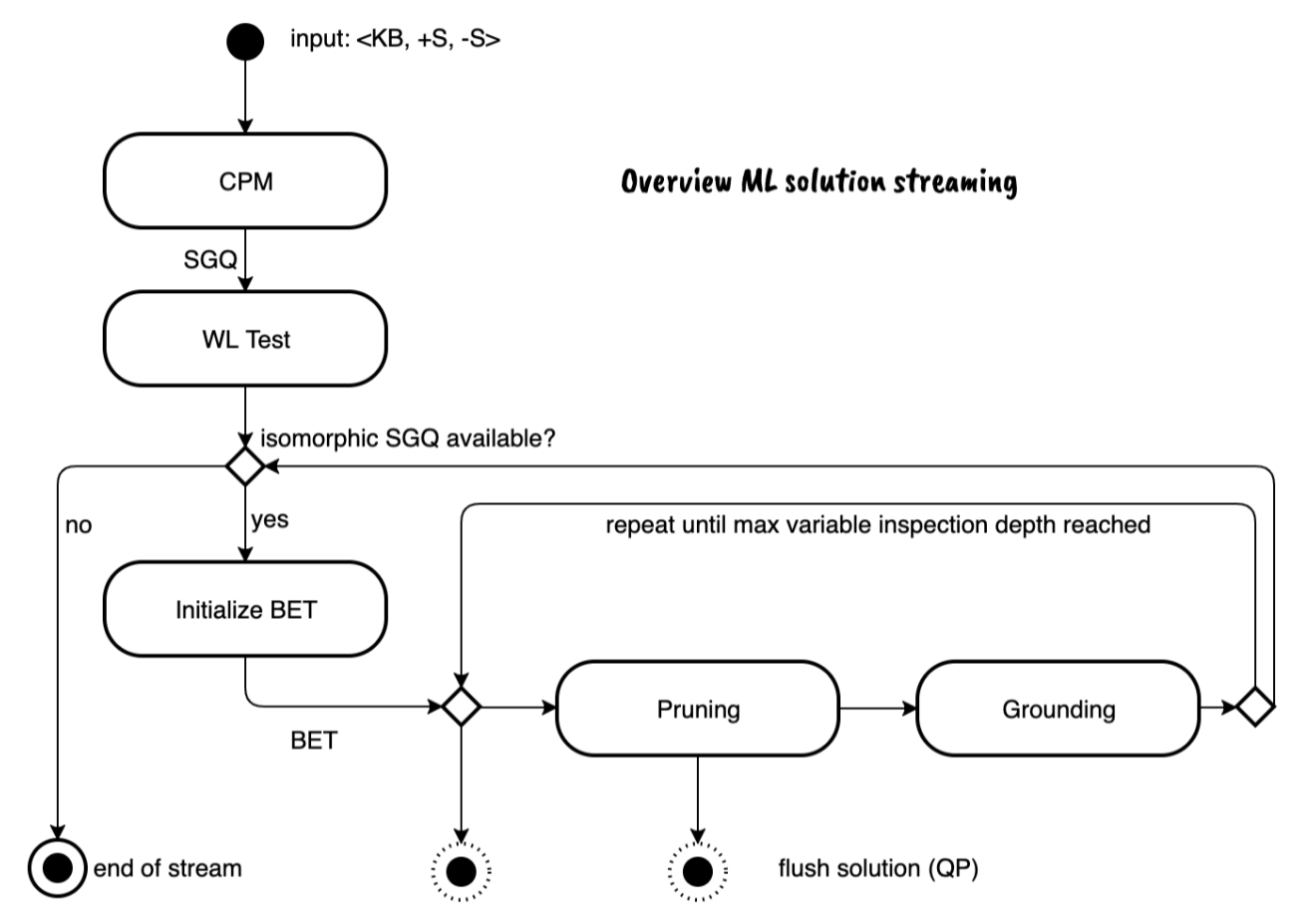
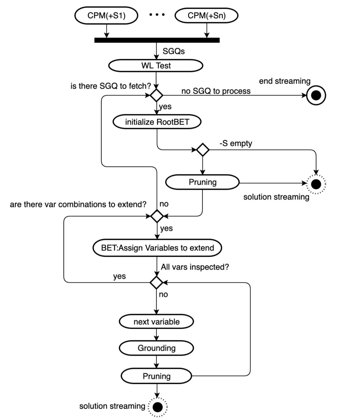
How the System Builds a Smart Search Program: A Step-by-Step Journey
The method follows an iterative process to refine the search program:
- Connecting the Dots (Connecting Path Module -
CPM):
◦ First, the system takes your positive examples (+S) and finds the smallest possible sub-graphs within the knowledge base where all the items in your positive sample are linked together.
◦ These sub-graphs are delivered in order, from the smallest to the largest. This part of the process is specially designed for hypergraphs and scales well even with very large databases. - Finding Similar Structures (Hypergraph Isomorphism):
◦ From all the sub-graphs found for your positive samples, the system then picks out the ones that have the same underlying structure.
◦ It uses a modified version of a smart algorithm called Weisfeiler-Leman (WL) to do this, which helps avoid incorrect matches and works efficiently. It’s important that this check only focuses on the variables that represent your sample items (likeX0,X1) to prevent errors. - Turning Structures into Queries (
SGQ):
◦ Once a similar structure is identified, it’s transformed into a generic query (SGQ).
◦ All the specific items in the graph are replaced with variables:
▪Xnfor the main items from your samples (e.g.,X0,X1).
▪Rnfor relationship types (e.g.,isA,partOf).
▪Anfor items that connect different parts of the query together.
◦ For example, if your positive samples were (berlin, germany) and (london, england), the system might create theSGQ:partOf(X0,X1),isA(X0,capital),isA(X1,country). - Running the Query and Checking Results:
◦ This generic query (SGQ) is then run against the knowledge base.
◦ This gives two “result tables” (RTs): one for the positive examples (+RT) and one for the negative examples (-RT).
◦ If the negative result table (-RT) is completely empty (meaning the query didn’t find any of your “unwanted” examples), then theSGQis considered a valid solution!.
◦ These results, along with theSGQ, are bundled together in a package called a “BET” (SGQ,+RT,-RT). - Refining the Query (Pruning):
◦ If the-RTis not empty (meaning the query still found some “unwanted” results), the Pruning phase begins.
◦ Its main goal is to find patterns in the result tables that clearly separate the positive examples from the negative ones. Then, it changes theSGQto filter out the negative samples.
◦ Strategies include:
▪ Variable Materialisation: If a specific value appears in all the positive results but none of the negative results for a certain variable, that variable in the query is replaced with that specific value. This makes the query more precise.
▪ Filtering: New logical rules are added to the query to explicitly exclude patterns found in the negative samples, likeA1 != 3ornot(has(X1, chlorophyll)). The system first looks for simple patterns before trying more complex ones.
▪ (A related technique, Variable Unification, adds rules to prevent variables from being equal if they consistently show up as equal in negative examples. This happens when new parts are added to the query during the next phase, Grounding). - Expanding the Search (Grounding):
◦ If Pruning isn’t enough, or to find more ways to refine the query, the Grounding phase steps in.
◦ This involves adding more detail and expanding theSGQ, including new nodes. It does this by asking the knowledge base for all the “neighbours” (connected items) of specific values found in the positive result table (+RT).
◦ These new items and their relationships are then incorporated into an extendedSGQ, along with new variables. This process enriches the data available, increasing the chances of finding clear differences during the Pruning phase.
◦ For negative samples, if the extended query doesn’t match the knowledge base, that negative row is removed from consideration.
The whole process works in cycles: BETs (the query, positive results, and negative results) are copied and refined through the Grounding and Pruning phases until a perfect solution is found. If no more options can be explored for a specific query type, the system moves on to the next, or stops if all possibilities are exhausted.
Hypergraph Isomorphism: A Key to Efficient Query Generation
You have two complex diagrams made of interconnected points and lines. How do you tell if they are fundamentally the same shape, even if they’re drawn differently or have different labels? This is the core challenge of graph isomorphism: determining if two graphs have an identical underlying structure. More formally, two graphs are isomorphic if you can find a unique function that perfectly maps the nodes of one graph to the nodes of the other.
In the context of this method, an intelligent variation of the Weisfeiler-Leman (WL) algorithm is employed to efficiently identify these structural similarities in hypergraphs. This ensures that the system can recognise the same underlying pattern in your positive examples, even if the specific items within them differ.
The Weisfeiler-Leman Algorithm: A Brief Overview
Two graphs are isomorphic when they have the same structure. In graphical terms, isomorphism is the property two graphs have if it is possible to arrange them such that they look the same.
A more accurate definition of isomorphism says that graphs are isomorphic when there is a function that can transform uniquely the nodes from graph G1 to the nodes of G2.
Here I present a variation of the Weisfeiler-Leman algorithm (WL) which lower considerably the chances of false positives, while keeping complexity at polynomial time. In the WL the nodes are assigned with a constant initial integer (ex.: 1) and then a reducing function (FI) is applied to each nodes and its neighbors for creating a new value associated to that node at that iteration. The process repeats until the sorting by the last iteration assignments, do not change the order of the nodes.
The modified function for calculating the value of a node $X$ at iteration $t$ is expressed as:
\[FI_t(X) = FI_{t-1}(X) + \sum_{E \in E_{incident}(X)} \left( w(type(E)) \cdot \sum_{pos} FI_{t-1}(Node(E, pos)) \cdot pos \right)\]Where:
• $FI_{t-1}(X)$ is the value of node $X$ from the previous iteration.
• $E_{incident}(X)$ represents all hyper-edges connected to node $X$.
• $w(type(E))$ is a constant, unique weight assigned to the type of hyper-edge $E$ (e.g., p might be 1, q might be 2, r might be 3).
• $Node(E, pos)$ refers to the node at a specific position pos within hyper-edge $E$.
• The sum over pos ensures that the position of a node within an edge influences its calculated value
As an example we have 2 graphs:
G1 = p(X0, X1, X2), q(X0, A0, X1), r(A0, X1, X2)
G2 = q(X1, A0, X0), r(A0, X0, X2), p(X1, X0, X2)
A constant unique weight is assigned to the edge type: p->1, q->2, r->3.
At the beginning (iteration T0), the aggregate map, for all terms, and for both G1 and G2, is set to 1:
| Node | T0 |
|---|---|
| X0 | 1 |
| X1 | 1 |
| X2 | 1 |
| B0 | 1 |
In the first iteration(T1), the FI function is applied to all nodes. There is corresponding mapping between nodes in G1 and G2:
| Node | G1 | G2 |
|---|---|---|
| X0 | 18 | 36 |
| X1 | 36 | 18 |
| X2 | 24 | 24 |
| A0 | 30 | 30 |
Nodes with same value in G1 and G2 columns are isomorphic.
Selected Variable Correspondence
A key challenge with isomorphism tests is that they might not differentiate between the “terminal” variables (like Xn, which represent your actual sample values) and “joining” variables (like An, which are just for connecting parts of the query). If not handled carefully, this could lead to false positives, where the algorithm mistakenly associates an An value from one dataset with an Xn value from another.
To prevent these errors, the isomorphism test within this method is only performed on the Xn variables. In the example table above, since there’s a correspondence of values for Xn variables (e.g., X0 in G1 maps to X1 in G2, and vice-versa), the isomorphism test between G1 and G2 is considered positive.
Once an isomorphic structure is identified among the sub-graphs of your positive samples, it can then be transformed into a generic query (SGQ). For instance, if your positive samples were (berlin, germany) and (london, england), and the system found them to be isomorphic, they could be transformed into the SGQ: R0(X0,X1)
Pruning
The Pruning phase is a crucial component of the in-memory hypergraph machine learning method, designed to refine the synthesised query program (QP) to accurately discriminate between +S and -S. It aims to ensure that when the QP is executed, it returns all +S while excluding all -S.
Pruning is performed if the Result Table (-RT), generated by executing the generic query (SGQ) against the KB for -S, is not empty. Its primary goal is to detect patterns in the data within the +RT -RT that can be used to differentiate -S marked rows from +S ones. If such a pattern is found, Pruning modifies the SGQ by unifying or materialising one or more variables, thereby adjusting the query to exclude the negative examples. If this initial pruning fails, new relational constraints are appended to the SGQ in a subsequent “Grounding” phase.
The system employs a couple of strategies to leverage analogies in the RTs data for pruning:
- Variable Unification: this tactic is activated if a pair of nodes shows equality in all -S rows. It then adds a specific constraint to the SGQ to disallow equalities in those variables.
- Variable Materialisation: if a variable appears in all
+RTrows but not in any-RTrows, then the corresponding variable in the SGQ is replaced with that specific value. This effectively narrows the scope of the query. - Filtering: If a common value is found among negative samples in a variable column that cannot be materialised for
+S(because+Srows don’t share a common value), then this common value can be excluded. This involves adding a new logical operation to theSGQ.
Connecting Path Module (CPM)
The CPM extracts a sub-graph from KB such that a set of nodes (terminals) are all linked. This is well known problem in graph theory called Steiner problem. The innovative algorithm is specifically designed for the setup encountered on this domain and in particular:
- It is designed for hypergraphs and therefore the reach of this method outclasses algorithms intended for generic graphs.
- The method does not return simply the smallest sub-graph, but it returns a stream of sub-graphs (in ascending order size).
- Differently from the Kruskal’s algorithm this algorithm does not mapping of all nodes in the graph as prescribed by the Dijkstra algorithm (used in Kruskal’s algorithm). This algorithm scale even in very large KB without sufferings due to the size of the target DB. The advantage is done in the terminal solver function (described below) which fetches the next node to visit and add to its internal queue all its neighbors that aren’t already visited.
The Real-World Impact: Fast, Intelligent Data Analysis
This method offers significant benefits, especially for data that naturally exists in discrete forms, such as in relational databases or graph databases.
Because it’s designed for in-memory computation, there’s no time wasted sending data back and forth over networks. This makes machine learning tasks much, much faster than other methods.
This incredible speed allows for “online” and “synchronous” machine learning operations. Imagine getting instant insights and generating queries on the fly, rather than waiting for slow batch processing. This capability has huge potential for quickly understanding and acting on constantly changing information in diverse fields.