Process modeling may be used to enhance the robustness and resilience of processes to unfavorable events, and to improve forecasts. Modeling complex processes may involve representing and evaluating long chains of time-dependent data values that depend on one another, for example, as cause-and-effect. Therefore, it is desirable for enterprises to model various complex business/technical processes.

One way to address these challenges is to employ analysts to generate process models using a spreadsheet or similar software tool. For example, the spreadsheet may be arranged with columns where different columns correspond to different times or different time periods. Although these techniques may generate accurate models when executed with great care, they are not user friendly and the manual creation of the models can consume considerable human resources.

Attaining expressive ergonomicity in structure representation is both crucial and challenging. The “make things simple but not simpler” principle guides all human-computer interface design, including temporal programming—a well-known concept in logic. I introduce syntactic sugar to enhance readability and express temporal context switching, a fundamental aspect in process analytics.

Case Study

Consider an example in which ACME Ltd executes a industrial process to manufacture a product. That dummy process may include various different steps and may incorporate raw materials are added from suppliers and retrieved from inventory during the process. The company receive purchase orders from customers, then they are processed according to the production capacity. Such process model should consider statistical deviations on planned deliveries due to unexpected situations (sick workers, or unavailabilities of any kind).

At the end of the fiscal year, ACME’s CEO requests the Strategic Analysis and Forecasts team to report about delivery and storage costs. Differently from previous analyses, the team setup a simple model about their manufacturing pipeline. The order status is categorized in submitted, processing, pending, processed, or delayed. At any quarter, they identify the number of items in each of the statues, for example in Q1 processing(X) tell us that X number of items are in building process in the manufacturing chains.

As depicted in the figure below, raw items are arriving from suppliers at each quarter, as well as orders and of course deliveries to customers.

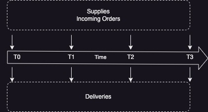
As any enterprise with fixed and variable costs, ACME stores items in rented warehouse blocks with precise storing spaces, such that the enterprise rent space according to its inventory at every quarter.
Now, let’s define some rules, such as:

availability(Supply + Inventory) ⟸ supply(Supply), <<inventory(Inventory)

which means ‘Available material depends on supply, and the inventory in the previous quarter’ in plain English. The << symbol stands for previous the time context, the time scale could be anything from milliseconds to ages. We have decided to reason on quarter base.
Next step on modelling will be on defining how items change status with time. Might be an over-simplification, but nobody will complain if we remark the actual productive throughput is the minimum between the productive capacity and stockpile. Could it be that currently, pending orders are the delayed and pending ones from previous quarter plus the new submitted, minus the actual processing orders? In ACME people believes so.

processing(Processing), 
pending(To-do - Processing), 
inventory(Available - Processing) 
	⟸ <<delayed(Delayed), 
	   <<pending(Pending), 
	   submitted(Submitted),
	   To-do = Delayed + Pending + Submitted, 
	   availability(Available),
	   capacity(Capacity),
	   min(Capacity, Available, Possible), 
	   min(To-do, Possible, Processing)

Unfortunately, not all orders are assembled on time. 1% are delayed to the next quarter by setting the parameter toDelay(.01).

Now it’s time to specify the cost of delivery:

costDelivery(Processed * Unitcost + PrevCostDelivery) 
	⟸ processed(Processed), 
	  singleDeliveryCost(Unitcost), 
	  <<costDelivery(PrevCostDelivery)

It’s time to run the model by specify constant parameters and time-based input such as:

Q1 -> supply(10), submitted(7),
Q2 -> supply(2), submitted(3)
Q3 -> supply(3), submitted(5)

And then query the model with ?costDelivery(DeliveryCost):

DeliveryCost = …

Time Clock

This approach show similarities with differential calculus, the branch of math that concern about solving equations that include functions dependent one to each other. An example is the determination of a ball fall velocity as function of time due to the gravity. The ball slow down by the friction with air, which increase when velocity increase slowing down the ball (in this case, it’s negative feedback). While the fall of ball could be calculated in closed form, simple yet chaotic processed (eg.: cellular automata) are solvable only by running the model. No shortcut available.

For time-based models, time is the ticker the governs the model evolution. Could be seen as the CPU Clock for your computer. As the clock triggers new computation due to the previous state of memory and the new instruction to be executed, a new time step in the modelled process affect the (virtual) state of a process. In the description:

on(Light) <= <<off(Light)
off(Light)<= <<on(Light)

I create a perpetual switching on/off translated as: if the light was off in T-1 then the light will be on and vice-versa.

System Dynamics

The study of dynamic processes that depends each other is an old branch of system theory which brings us some fancy graphical representations like the one below that relates economy, gas emissions, population and social issues:

I quote from Wikipedia:

The basis of the method is the recognition that the structure of any system, the many circular, interlocking, sometimes time-delayed relationships among its components, is often just as important in determining its behavior as the individual components themselves

Conclusion

The symbol ‘«’ is a syntactic sugar for the more verbose event calculus, a temporal based logic semantics, where specialized predicates specify whether an Event occurs at a specific time T with holdsAt(Event, T), or persist indefinitely after T with initiates(Event, T) or cease to exists at certain time terminates(Event, T).
The temporal context-switching relies on dynamic programming by visiting all temporal contexts backward (or forward) until the beginning of time (or the end). The advantage of dynamic programming is memoization (or tail call) for optimizing tree searches by caching contexts. The disadvantage is that temporal contexts should not change overtime. Changing the underlying data base during backtracking might incur in inconsistencies.