Dynamic Programming

The term dynamic programming has a curious origin.
When Richard Bellman late in the 1940s were seeking for a viral definition of his method, his boss was apparently not very inclined on science and in particular on mathematical research, the activities that Bellman was deep into when he formulate his famous equation.
Likewise in marketing campaigns, where names and terms are carefully selected for attention teasing, Bellman coined the definition that combines the multi-staging and time-varying of ‘dynamic’ with the optimization archetyping of ‘programming’, coincidentally induced by the fame of Dantzig’s linear programming for mathematical optimization.

DP describes problems that involve dynamic processes for finding the best decision one after another. The backbone idea rolls around the splitting of a problem till its atomic parts are identified, then trimming those parts with a objective function. Basically, the core concept of recursion. Considering for example the Fibonacci algorithm:

The node fib(2) appear twice in the tree, therefore Fibonacci unveils an overlapping structure. It is eligible to be an DP algorithm. Not all recursive algorithms are inherently overlapping, look at binary tree search, merge and quick sort, for example. They don’t manifest the property of traversing smaller chunk of data more then once, hence they cannot join Dynamic Programming’s family. When the sub-problems are repeated in the problem as whole, and their values are evaluated all over again unless a caching mechanism (memoization) could be displaced for preventing such inefficiency.

Bellman also conceived the principle of optimality according to which an optimal policy should always hands out the optimal decision from any state or action previously done. However the chessboard pieces’ are laid, or however pedestrian are crossing the road or waiting on the platform, the agent will move pieces properly in case of chess and it will skirt traversing people in case of self-driving car. The automatic actor will always follow the best strategy from the first step and thereafter.
This is for introducing another property of DP methods, which is the optimal structure.

When a courier has to deliver a packet from \(A\) to the destination \(F\), he will catch the shortest way highlighted in blue. The optimal decision for completing the journey \(A \rightarrow F\), in the shortest path problem, includes necessarily the optimal solution \(C \rightarrow F\). As you may have noticed, The recursion sweats also out of this property where nested sub-problems are always optimal on their way to the final target. The shortest path problem present the optimal sub-structure, which claims that an optimal solution of a problem includes necessarily the optimal solutions of its sub-problems. Not all recursive problems are optimal even in their encapsulated structure, and the counterfactual is given by slightly different dilemma, the longest path problem. The longest way \(A \rightarrow F\) includes the node \(C\), but if we choose to start from \(C\), the path is not included in the way starting from \(A\).

Dynamic programming in reinforcement learning

The first time DP and RL were mentioned together was by Minsky in the 1961 and it took form of the Bellman equation, because RL problems have expose usually an overlapping and optimal structure, ideal for being solved by DP.

Markov decision process

Reinforcement learning is a class of methods for determining the optimal policy an agent should apply for maximize its return in a given environment. The entities with a role in RL are the state \(S\), the mutable conditions an agent experience in an environment, the action \(A\) the agent execute in a particular state, and the reward \(R\), if any, which score the goodness of action taken in a state. These are the pillars of the markov decision process, the framework that formalizes the policy \(π\) as a sequence of steps \((S_t, A_t, R_t)\), aggregated in episodes.

The policy is a mapping from states and related actions, RL tells us how the agent’s policy changes as result of the experience.
For finding good policies, we need to estimate how good it is, in terms of future rewards, to be in a particular state. Value functions \(v_\pi(s)\) define the expected return when starting from a given state \(s\) and following \(\pi\) thereafter. their fundamental property is that they satisfy recursive relationships similar to what we already have seen for dynamic programming. Hence, the idea of DP in RL is the use of value functions to organize the search for good policies.

The Gridworld example

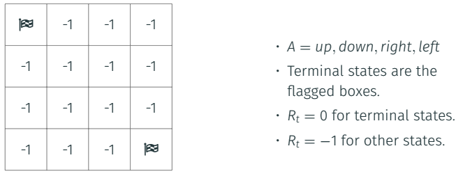
Problem: Find all trajectories towards the flags from any cell

Among many examples I may show for explaining what does DP stands for, this very simple GridWorld conveys the idea of an agent displaced in an 2D environment. The reward drives the agent to move toward the flagged corners regardless the position where the agent is located.
How the agent could learn the optimal ways? I give you an hint, let’s start from the end, the flagged boxes.
In that position you don’t have anymore rewards to gather, the task is brilliantly completed, so we assume the terminal’s state value is is equal to zero.

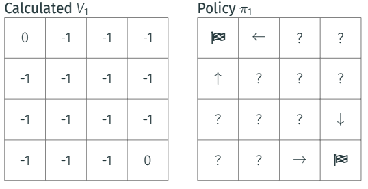
Iteration 1. Terminal state value is zero

From end position, step back and look around. Among the actions you can do, the move that catapult you into the terminal state is more rewarding than others (zero instead of -1).
Congratulations! You already have solved a piece of the puzzle. It is just the last action, you still have to solve the rest of the grid. In that position, as in any other cell of the grid, you need to assign a value to the cell where you are in that particular moment, in order to pave the way to the final goal. That value \(Q\) indicates how good it is to be there. Not all cells carry the same value, some are more valuable than others. The agent, when choosing the next move, will move to the cell with highest value, among the surroundings. The value would not be just the reward you get in there (-1), but the reward plus the average of the values of the cells proximate to you.
\(Q_t = r_t + \sum_{n=t+1}{Q_n}\)

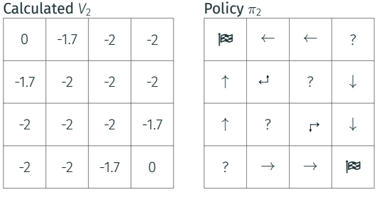
Iteration 2: set the terminal state value to _zero_

Going backward till the initial position, you see all rewards on the way to the terminal state waiting for you to being picked up. This is the value of your state.
You are in the middle of the trajectory towards the end, and the value of your state is equal of the reward in that state plus the sum of the discounted rewards thereafter.
Clearly, the agent moves toward the most promising among the surrounding cells, once it has realized their value. Let’s keep going.
The grid starts to unveil the optimal trajectories by just going backward and evaluating what could be the best move, taking the cell with highest value.
A pattern is identifiable, something that programmers knows well, the recursion, and simplified as: