Spectral Neural Networks for Knowledge Graphs (in Scala)
The power of networks. Metaphors of our collective life, with all of its complexity and its entangled dependencies.
Two types of networks, the network of data and the network of artificial neurons when combined together open the way to a variety of interesting applications. Typical examples of data networks include social networks and the knowledge graphs, while, on the other hand, a new family of machine learning tasks based on neural networks has grown in the last few years. This lineage of deep learning techniques lay under the umbrella of graph neural networks (GNN) and they can reveal insights hidden in the graph data for classification, recommendation, question answering and for predicting new relations among entities. Do you want to know more about them?
When we talk of machine learning tasks, we refer to a set of algorithms that finds correlation between input and output. The input is basically a list of numbers also known as vectorized features:
| Symbol | Vector representation |
|---|---|
| hiking | 0.12, 0.25, 0.66, 0.45 |
| mountain | 0.16, 0.29, 0.62, 0.40 |
| seaside | 0.02, 0.70, 0.39, 0.60 |
The vector representation of the nodes in the knowledge graph should preserve, to the maximum extent, the information carried by the single node within its own attributes compressed in a low dimensional space. In other words, the embeddings (the name of the vectorized representation) should identify the related symbol with a vector, and such vectors should be as small as possible. The objective of this article is about to find a proper way to generate good embeddings out of knowledge graphs.
For being useful in downstream machine learning tasks, embeddings should not just identify the related symbol but also they should have an important property. Symbols that are similar to each other – for whatever criteria we define for ‘similarity’ – should be associated with embeddings that are also similar, according to the favorite distance functions. In the above example, Hiking embeddings are more closely related to Mountain rather than Seaside. Embeddings are very familiar for those practiced in natural language processing, and they are based on the principle “a word is characterized by the company it keeps (R. Firth)”, and the skip-gram technique is employed for predicting what is the most likely word surrounded by a given set of predecessors and successors. Applied to a huge corpora, the trained skip-gram (or its complementary cbow) network will contain the embeddings that fulfill the similarity property. While the words in a text are strictly in sequential order (with one predecessor and one successor), in a graph a node might hold a multitude of relations, and as if that is not enough, those relations might be different one to another.
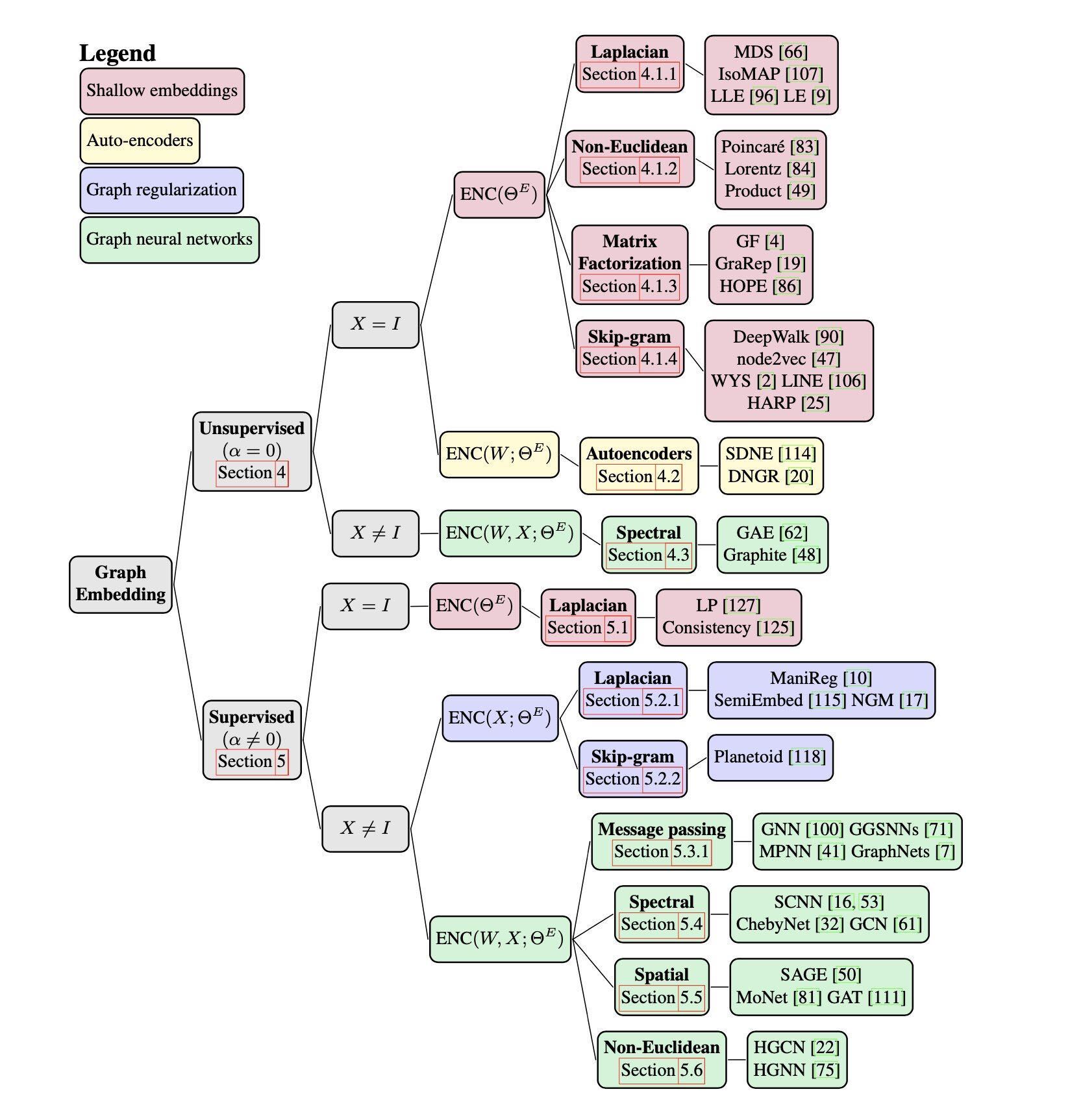
Representation learning is flourishing and new approaches are invented at an increasing rate:

Hereafter, I will present just two techniques for generating embeddings in graphs. For the sake of statistics, I implemented Deepwalk and Graph convolutional networks (GCN) in Scala with ND4J for matrices, and Deeplearning4J as a neural network framework.
Deepwalk algorithm
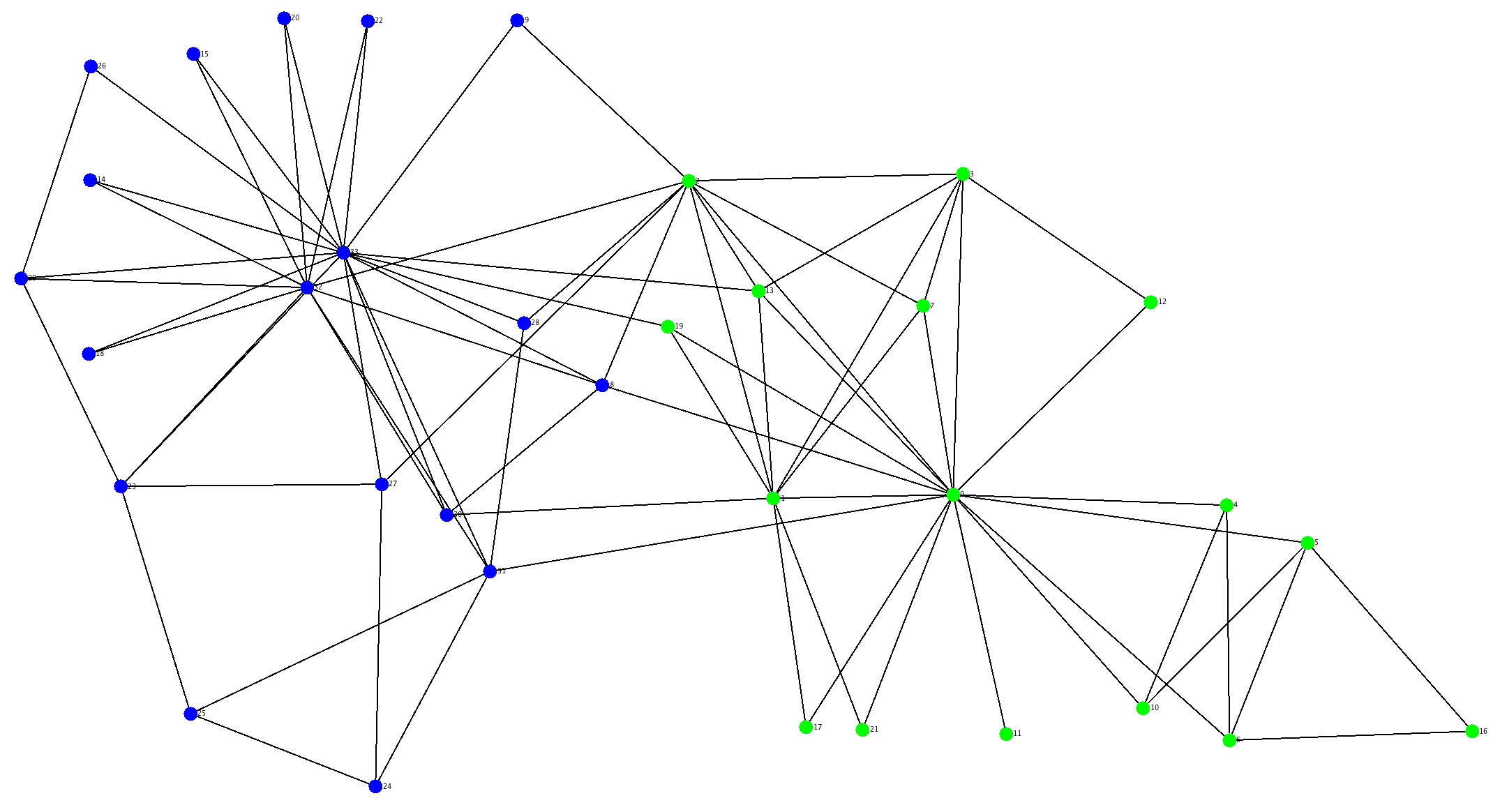
The Deepwalk (and its successor Node2Vec) is an unsupervised algorithm, one of the first in the realm of representation learning for graphs, and it is as simple in its design as it is effective on capturing topological and content information. In principle it is equivalent to the already mentioned skip-gram, but how can the graph structure match the streaming sequence of words in a text? Starting from any node of choice, the algorithm visits its neighbors and the entire network in a controlled random way. The random walk is balanced among two different approaches that emphasize differences in closely related nodes in one case, and the differences among distant clusters in the other. The first approach is the Breadth First Search (BFS) which selects the next node to visit among the siblings of the current node, in the respect of the previous node. The second approach is the Deep First Search (DFS) that selects the new node among the connected nodes with the current one. The first persists with all neighbors of the current node, while the second tends to explore the network in depth.

What are the Graph Convolutional Networks?
The graph convolutional networks, as the name might recall, share some commonalities with the convolutional neural network algorithm, the one that led the way to giant leaps in visual recognition. If a graph with nodes and edges is transposed in a two dimensional adjacent matrix, nothing can prevent us from running a sliding window function that compresses a grid of pixels and extracts features like CNNs do. The affinity with CNN ends here, because when we elaborate images we are more interested in complex visual features rather than single pixels. In knowledge graphs, on the other hand, we want to convolute in a single node its neighbours and recursively the information of the entire network.
The Weisfeiler-Lehman Test
The principle underlying GCNs lay its fundations on a method described several decades ago in the Weisfeiler-Lehman test. The test would determine whether two arbitrary graphs are isomorphic, i.e. they have exactly the same structure. According to the algorithm, all nodes are initialized with the same value, let’s put number 1 for all. Then, to that node is assigned that value plus the value of its neighbors, and this step is iterated. As you might think, in the first round the node already includes the information of first degree neighbors, but at the second iteration, the node will get a distilled notion of the second line of nodes, and so on as the iterations proceed. The test will confirm the isomorphism whether, after an arbitrary number of iterations, the partition of nodes by their current value does not change. Even though the isomorphism problem is not yet solved and the test is an heuristic attempt, the method brings the way to iteratively convolve information among the nodes.
The Spectral Propagation Rule
The GCN method is described in Kipf & Welling (ICLR 2017) and lies in the messaging passing methods family, whereas with “message” we intend solely the content of a single node and “passing” is the convolution which percolates throughout the network. While in the Weisfeiler-Lehman test the way to pass information is just a simple sum of values, in GCNs the convolution relies on the spectral propagation rule. What is this propagation rule? Let’s assume we know the graph structure (nodes and relations) and the content of all nodes (features). The propagation rule is applied with a linear matrix multiplication, but for not incurring in vanishing or exploding gradients in the downstream tasks, the features are normalized and a self-loop in the adjacency matrix is added.
import org.nd4j.linalg.factory.Nd4j._

def spectralLayer(adjacent: INDArray, input: INDArray, weights: INDArray):INDArray {
  //add self-loops
  val ah = adjacent.add(eye(adjacent.columns()))
  val ssm = create((0 until ah.rows).map(ii => ah.getRow(ii).sumNumber().floatValue())).toArray
  //normalization
  val spectre = diag(pow(ssm, -.5))
  //non linear-function (relu) to the spectral Rule
  relu(spectre.mmul(ah).mmul(spectre).mmul(input).mmul(weights))
}
// the first layer takes a diagonal input and random weights
val l1 = spectralLayer(adjacentMat, eye(nodes.length), rand(nodes.length, 4))

// the second layer takes l1 as input and random weights
val out = spectralLayer(akat, l1, rand(l1.shape()(1).toInt, 2))
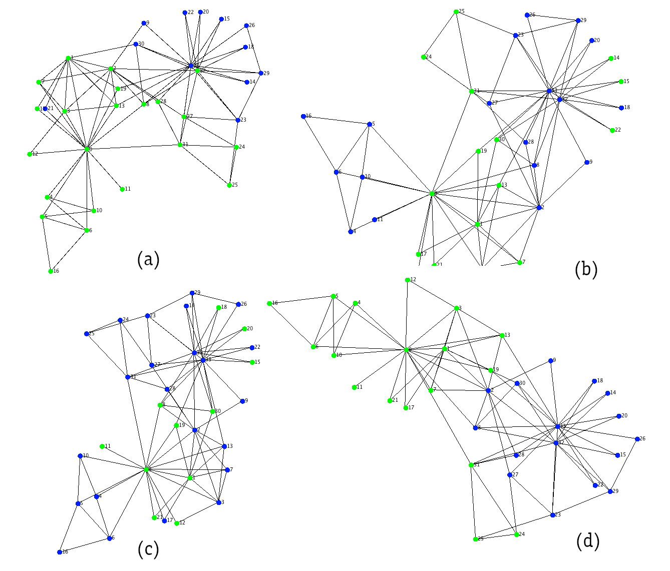
I created some experiments with the small karate dataset, a fake set of node features (just a diagonal matrix) and a random set of weights. I repeated 4 experiments in sequence (no cherry-picking) in the image below where the color of the nodes indicates their similarity after running 2 iterations of the spectral algorithm.

The results are clearly amazing! The two clusters are yet unrefined but as you can see the figure (d) is almost exactly what we obtained with Deepwalk! Those embeddings are elaborated with just random weights and 2 recursive iterations. Why not apply some learning mechanism for refining the clusterization with few examples?
Semi-supervised Learning with GCNs
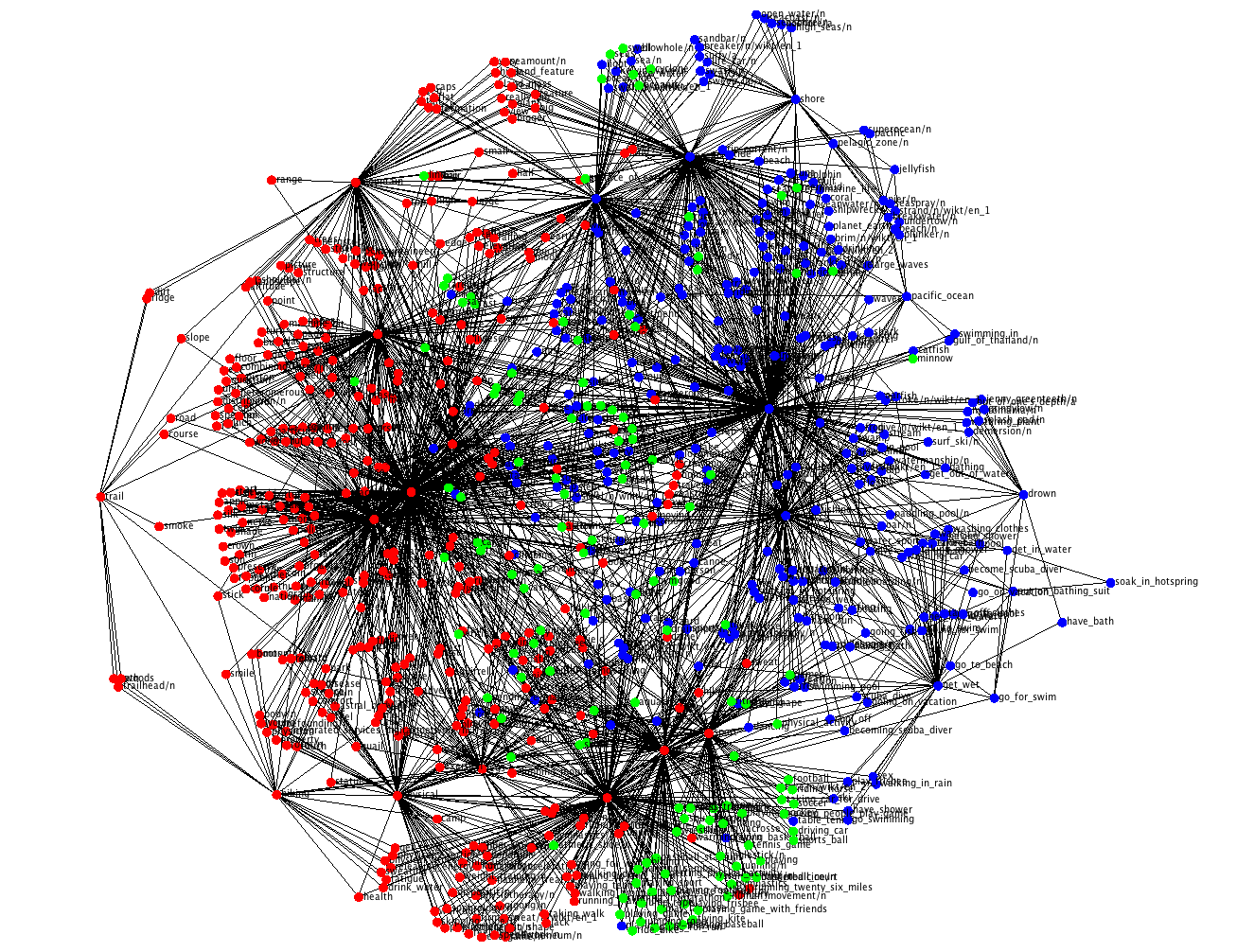
I started this post on how your e-commerce could recommend new items according to your customers’ holiday preferences and I’ll run some experiments with a more pertinent dataset. If you are not familiar with ConceptNet, it is a huge graph database of general facts with 34 millions nodes, 34 types of different relations that I converted entirely in a OWL database. I extracted approximately 3 thousands of nodes about our topics of interest, the mountain and the seaside. Then I created a 2-layered neural network with the spectral propagation rule. I fed it with the adjacency matrix, the word-embeddings of the node names as input features and some labelled nodes. Two nodes classified as “seaside” category, and two nodes classified as “mountain” category. The 4 labelled nodes with 2 categories is all I need for classifying all the rest of the 3 thousands labels. That’s a ratio of 4/3000 labelled entries in the respect of the entire dataset, isn’t interesting? That’s why the name semi-supervised learning.

This method of classification is really fast but has some drawbacks. The spectral propagation rule takes into account the adjacency matrix which is the whole network in a two dimensional vector. For a relatively small dataset that’s not an issue, but when it comes with real big data this method is actually unfeasible. The FastGCN comes into the rescue and scales to big sized graph DBs.
Comments